Tanaka (illuminated) contours

[argyris]

Hello everyone!

I am interested in implementing Tanaka (illuminated) contours just like in the image below:

My logic is the following:

1. Extract the line contours as segments
2. Compute the normal vector at each segment
3. Compute the angle between the normal vector and light source
4. Change the width and colour of the segment based on the angle. So if the segments point to the light source it should become white and thinner, if they point away black and thicker, as Tanaka proposed.

I would appreciate any help on how to implement this algorithm in matplotlib.
I think my main issue is how can I extract the contour lines and discretise them in order to compute the normal vector and change afterwards the colour and width of the line.

Thank you in advance!

Argyris

[ianthomas23]

Hi Argyris,

Here is an example of how to extract points from line contours:

import matplotlib.pyplot as plt
import numpy as np

n = 5
x, y = np.meshgrid(np.linspace(0, 1, n), np.linspace(0, 1, n))
z = np.exp(-(x-0.5)**2 - (y-0.5)**2)

fig, ax = plt.subplots()
cs = ax.contour(x, y, z, levels=[0.75, 0.9])
for level, collection in zip(cs.levels, cs.collections):
    segments = collection.get_segments()
    print(f'z-level {level} consists of {len(segments)} line(s)')
    for line in segments:
        # 'line' is an array of shape (?, 2).
        # May be closed (last point == first point) or open.
        print(f'  shape {line.shape}, closed {np.all(line[0]==line[-1])}')

This produces the following output:

z-level 0.75 consists of 4 line(s)
  shape (4, 2), closed False
  shape (4, 2), closed False
  shape (4, 2), closed False
  shape (4, 2), closed False
z-level 0.9 consists of 1 line(s)
  shape (13, 2), closed True

From here you can use each line (2D array of points) to work out your normal vectors, etc.

Drawing the lines in matplotlib with the colour and width varying along the line will be awkward. Matplotlib expects a line to have constant colour and width, so you will have to break up each line into a number of sublines over which the colour and width are constant. You could draw them at the same time using a single LineCollection object, see matplotlib.collections — Matplotlib 3.3.3 documentation

[argyris]

Thanks for the reply Thomas, I think I did it in a slightly different way.

Here is my code:

import matplotlib.pyplot as plt
import numpy as np
from matplotlib.collections import LineCollection
from mpl_toolkits.mplot3d import axes3d

# Normalize vector
def normalize(X):
    return X / (1e-16 + np.sqrt((np.array(X) ** 2).sum(axis=-1)))[..., np.newaxis]

# get data
X, Y, Z = axes3d.get_test_data(0.02)

fig, ax = plt.subplots()

cs = plt.contour(X, Y, Z, levels=14, colors='None')
plt.contourf(X, Y, Z, levels=14, cmap="Blues")

# Get contour segments
segs = cs.allsegs
# number of contour levels
num_levels = len(cs.allsegs)

# LightSource direction 225deg
ls = np.array([-np.sqrt(2)/2, -np.sqrt(2)/2])

# Loop through levels
for lvl in range(num_levels):

    # Loop through elements on each level
    for el in range(len(cs.allsegs[lvl])):

        # Get segment from level=lvl and element=el
        xn = cs.allsegs[lvl][el][:, 0]
        yn = cs.allsegs[lvl][el][:, 1]
        points = np.array([xn, yn]).T.reshape(-1, 1, 2)
        segments = np.concatenate([points[:-2], points[1:-1],points[2:]], axis=1)

        # Compute normal vector from segments
        dy = segments[:, 1, 1] - segments[:, 0, 1]
        dx = segments[:, 1, 0] - segments[:, 0, 0]
        N = normalize(np.column_stack([-dy,dx]))

        # Compute cosine of angle theta between normal and lightsource
        costheta = -np.dot(N, ls)

        # LineWidths based on cos(theta)
        lwidths = np.abs(0.7 * costheta)

        lc = LineCollection(segments, linewidths=lwidths, cmap="Greys", norm=plt.Normalize(-1, 1))
        
        # Color based on cosine
        lc.set_array(costheta)

        ax.add_collection(lc)

plt.savefig('tanaka.png', dpi=600)

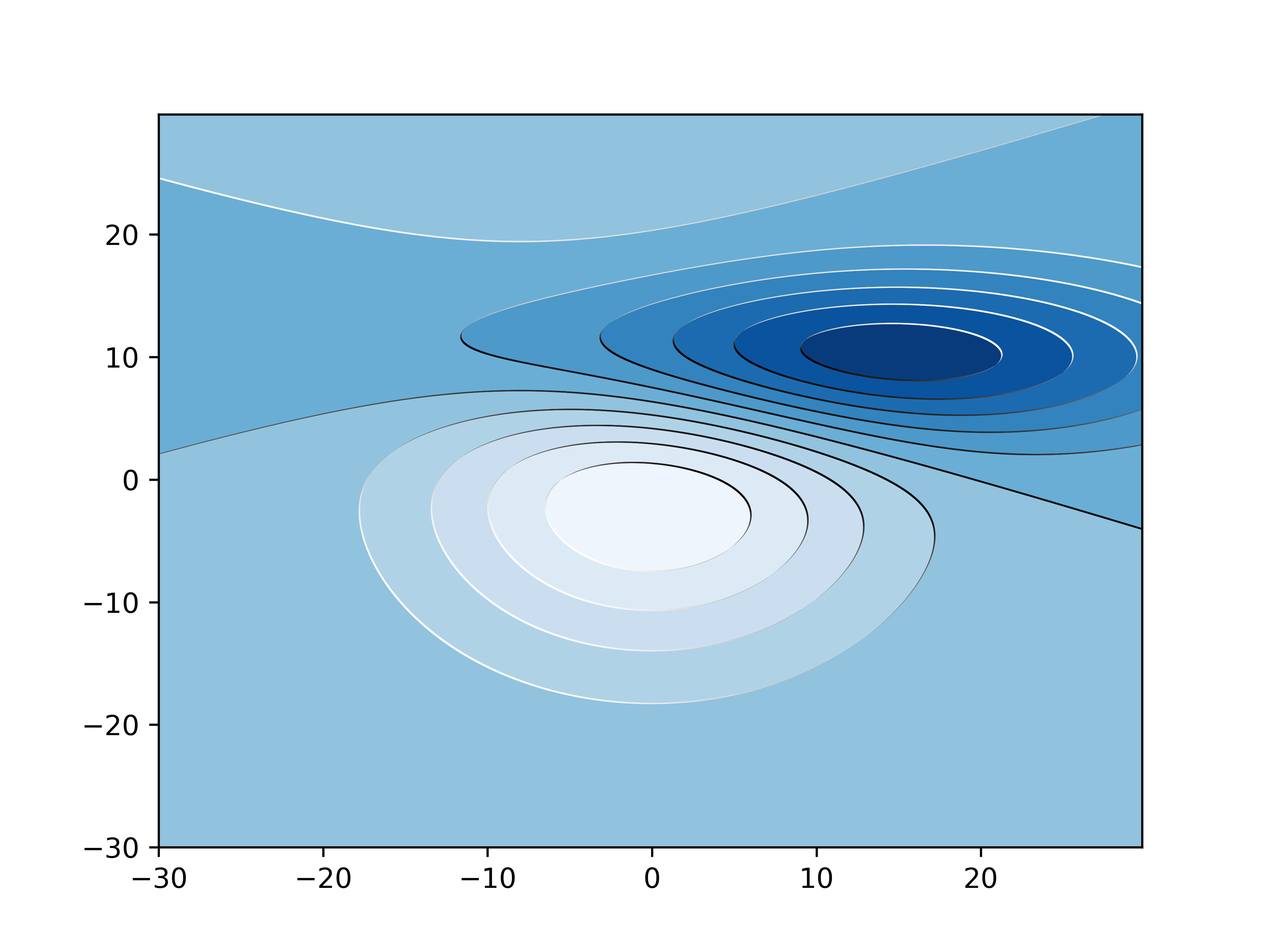
And here is the resulting image:

It works pretty well, perhaps two points of improvement might be:

1. getting the contour line collection without having to plot the contour
2. the linecollection isn’t a smooth curve so if you zoom in you might see discontinuities between each segment.

Thanks again.

[jklymak]

Matplotlib has hill shading in the 3D toolbox. So if you can make your contours a surface you will get the annoying light and perspective calculations for free.

[argyris]

Yes, I thought of starting with hillshading, but I couldn’t find a way to use it for producing the image above. I will have another look, thanks for the suggestion.