The code below works perfectly. I think this should be included as an
mplot3d codex. I'll look into what's required to submit a new example
to the documentation.
Thanks Armin!
···
Jeff Klukas, Research Assistant, Physics
University of Wisconsin -- Madison
jeff.klukas@...3030... | jeffyklukas@...3031... | jeffklukas@...3032...
http://www.hep.wisc.edu/~jklukas/
On Thu, Mar 18, 2010 at 9:42 AM, Armin Moser <armin.moser@...2495...> wrote:
Hi,
you can create your supporting points on a regular r, phi grid and
transform them then to cartesian coordinates:from mpl_toolkits.mplot3d import Axes3D
import matplotlib
import numpy as np
from matplotlib import cm
from matplotlib import pyplot as plt
step = 0.04
maxval = 1.0
fig = plt.figure()
ax = Axes3D(fig)# create supporting points in polar coordinates
r = np.linspace(0,1.25,50)
p = np.linspace(0,2*np.pi,50)
R,P = np.meshgrid(r,p)
# transform them to cartesian system
X,Y = R*np.cos(P),R*np.sin(P)Z = ((R**2 - 1)**2)
ax.plot_surface(X, Y, Z, rstride=1, cstride=1, cmap=cm.jet)
ax.set_zlim3d(0, 1)
ax.set_xlabel(r'\\phi\_\\mathrm\{real\}')
ax.set_ylabel(r'\\phi\_\\mathrm\{im\}')
ax.set_zlabel(r'V\(\\phi\)')
ax.set_xticks()
plt.show()hth
Arminklukas schrieb:
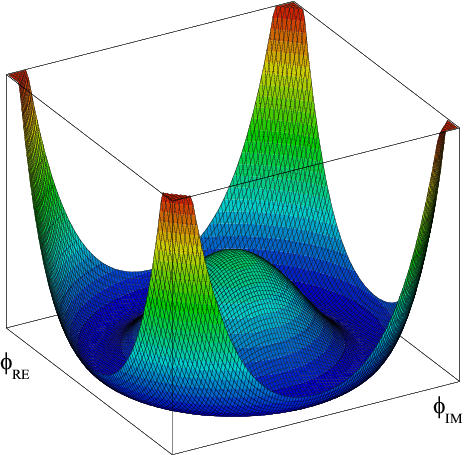
I'm guessing this is currently impossible with the current mplot3d
functionality, but I was wondering if there was any way I could generate a
3d graph with r, phi, z coordinates rather than x, y, z?The point is that I want to make a figure that looks like the following:
http://upload.wikimedia.org/wikipedia/commons/7/7b/Mexican_hat_potential_polar.svgUsing the x, y, z system, I end up with something that has long tails like
this:
http://upload.wikimedia.org/wikipedia/commons/4/44/Mecanismo_de_Higgs_PH.pngIf I try to artificially cut off the data beyond some radius, I end up with
jagged edges that are not at all visually appealing.I would appreciate any crazy ideas you can come up with.
Thanks,
JeffP.S. Code to produce the ugly jaggedness is included below:
-------------------------------------------------------
from mpl_toolkits.mplot3d import Axes3D
import matplotlib
import numpy as np
from matplotlib import cm
from matplotlib import pyplot as pltstep = 0.04
maxval = 1.0
fig = plt.figure()
ax = Axes3D(fig)
X = np.arange(-maxval, maxval, step)
Y = np.arange(-maxval, maxval, step)
X, Y = np.meshgrid(X, Y)
R = np.sqrt(X**2 + Y**2)
Z = ((R**2 - 1)**2) * (R < 1.25)
ax.plot_surface(X, Y, Z, rstride=1, cstride=1, cmap=cm.jet)
ax.set_zlim3d(0, 1)
#plt.setp(ax.get_xticklabels(), visible=False)
ax.set_xlabel(r'\\phi\_\\mathrm\{real\}')
ax.set_ylabel(r'\\phi\_\\mathrm\{im\}')
ax.set_zlabel(r'V\(\\phi\)')
ax.set_xticks()
plt.show()--
Armin Moser
Institute of Solid State Physics
Graz University of Technology
Petersgasse 16
8010 Graz
Austria
Tel.: 0043 316 873 8477