Recently, I had a need for a monotonic piece-wise cubic Hermite interpolator. Matlab provides the function “pchip” (Piecewise Cubic Hermite Interpolator), but when I Googled I didn’t find any Python equivalent. I tried “interp1d()” from scipy.interpolate but this was a standard cubic spline using all of the data - not a piece-wise cubic spline.
I had access to Matlab documentation, so I spent a some time tracing through the code to figure out how I might write a Python duplicate. This was an massive exercise in frustration and a potent reminder on why I love Python and use Matlab only under duress. I find typical Matlab code is poorly documented (if at all) and that apparently includes the code included in their official releases. I also find Matlab syntax “dated” and the code very difficult to “read”.
Wikipedia to the rescue.
Not to be deterred, I found a couple of very well written Wikipedia entries, which explained in simple language how to compute the interpolant. Hats off to whoever wrote these entries – they are excellent. The result was a surprising small amount of code considering the Matlab code was approaching 10 pages of incomprehensible code. Again - strong evidence that things are just better in Python…
Offered for those who might have the same need – a Python pchip() equivalent ==> pypchip(). Since I’m not sure how attachments work (or if they work at all…), I copied the code I used below, followed by a PNG showing “success”:
···
pychip.py
Michalski
20090818
Piecewise cubic Hermite interpolation (monotonic…) in Python
References:
Wikipedia: Monotone cubic interpolation
Cubic Hermite spline
A cubic Hermte spline is a third degree spline with each polynomial of the spline
in Hermite form. The Hermite form consists of two control points and two control
tangents for each polynomial. Each interpolation is performed on one sub-interval
at a time (piece-wise). A monotone cubic interpolation is a variant of cubic
interpolation that preserves monotonicity of the data to be interpolated (in other
words, it controls overshoot). Monotonicity is preserved by linear interpolation
but not by cubic interpolation.
Use:
There are two separate calls, the first call, pchip_init(), computes the slopes that
the interpolator needs. If there are a large number of points to compute,
it is more efficient to compute the slopes once, rather than for every point
being evaluated. The second call, pchip_eval(), takes the slopes computed by
pchip_init() along with X, Y, and a vector of desired "xnew"s and computes a vector
of "ynew"s. If only a handful of points is needed, pchip() is a third function
which combines a call to pchip_init() followed by pchip_eval().
import pylab as P
#=========================================================
def pchip(x, y, xnew):
# Compute the slopes used by the piecewise cubic Hermite interpolator
m = pchip_init(x, y)
# Use these slopes (along with the Hermite basis function) to interpolate
ynew = pchip_eval(x, y, xnew)
return ynew
#=========================================================
def x_is_okay(x,xvec):
# Make sure "x" and "xvec" satisfy the conditions for

# running the pchip interpolator
n = len(x)
m = len(xvec)
# Make sure "x" is in sorted order (brute force, but works...)
xx = x.copy()
xx.sort()
total_matches = (xx == x).sum()
if total_matches != n:
print “*” * 50
    print "x_is_okay()"

    print "x values weren't in sorted order --- aborting"

    return False

# Make sure 'x' doesn't have any repeated values
delta = x[1:] - x[:-1]
if (delta == 0.0).any():
print “*” * 50
    print "x_is_okay()"

    print "x values weren't monotonic--- aborting"

    return False

# Check for in-range xvec values (beyond upper edge)
check = xvec > x[-1]
if check.any():
print “*” * 50
    print "x_is_okay()"

    print "Certain 'xvec' values are beyond the upper end of 'x'"
print "x_max = ", x[-1]
indices = P.compress(check, range(m))
print "out-of-range xvec’s = ", xvec[indices]
    print "out-of-range xvec indices = ", indices

    return False

# Second - check for in-range xvec values (beyond lower edge)
check = xvec< x[0]
if check.any():
print “*” * 50
    print "x_is_okay()"

    print "Certain 'xvec' values are beyond the lower end of 'x'"
print "x_min = ", x[0]
indices = P.compress(check, range(m))
print "out-of-range xvec’s = ", xvec[indices]
    print "out-of-range xvec indices = ", indices

    return False

return True
#=========================================================
def pchip_eval(x, y, m, xvec):
# Evaluate the piecewise cubic Hermite interpolant with monoticity preserved
#    x = array containing the x-data

#    y = array containing the y-data

#    m = slopes at each (x,y) point [computed to preserve monotonicity]

#    xnew = new "x" value where the interpolation is desired
#    x must be sorted low to high... (no repeats)

#    y can have repeated values
# This works with either a scalar or vector of "xvec"
n = len(x)
mm = len(xvec)
############################

# Make sure there aren't problems with the input data

############################
if not x_is_okay(x, xvec):
    print "pchip_eval2() - ill formed 'x' vector!!!!!!!!!!!!!"

    # Cause a hard crash...
STOP_pchip_eval2
Find the indices “k” such that x[k] < xvec < x[k+1]
# Create "copies" of "x" as rows in a mxn 2-dimensional vector
xx = P.resize(x,(mm,n)).transpose()
xxx = xx > xvec
# Compute column by column differences
z = xxx[:-1,:] - xxx[1:,:]
# Collapse over rows...
k = z.argmax(axis=0)
# Create the Hermite coefficients
h = x[k+1] - x[k]
t = (xvec - x[k]) / h[k]
# Hermite basis functions
h00 = (2 * t3) - (3 * t2) + 1
h10 = t3 - (2 * t2) + t
h01 = (-2* t3) + (3 * t2)
h11 = t3 - t2
# Compute the interpolated value of "y"
ynew = h00y[k] + h10hm[k] + h01y[k+1] + h11hm[k+1]
return ynew
#=========================================================
def pchip_init(x,y):
# Evaluate the piecewise cubic Hermite interpolant with monoticity preserved
#    x = array containing the x-data

#    y = array containing the y-data
#    x must be sorted low to high... (no repeats)

#    y can have repeated values
# x input conditioning is assumed but not checked
n = len(x)
# Compute the slopes of the secant lines between successive points
delta = (y[1:] - y[:-1]) / (x[1:] - x[:-1])
# Initialize the tangents at every points as the average of the secants
m = P.zeros(n, dtype=‘d’)
# At the endpoints - use one-sided differences
m[0] = delta[0]
m[n-1] = delta[-1]
# In the middle - use the average of the secants
m[1:-1] = (delta[:-1] + delta[1:]) / 2.0
# Special case: intervals where y[k] == y[k+1]

# Setting these slopes to zero guarantees the spline connecting

# these points will be flat which preserves monotonicity
indices_to_fix = P.compress((delta == 0.0), range(n))
print "zero slope indices to fix = ", indices_to_fix
for ii in indices_to_fix:
m[ii] = 0.0
m[ii+1] = 0.0
alpha = m[:-1]/delta
beta = m[1:]/delta
dist = alpha2 + beta2
tau = 3.0 / P.sqrt(dist)
# To prevent overshoot or undershoot, restrict the position vector

# (alpha, beta) to a circle of radius 3.  If (alpha**2 + beta**2)>9,

# then set m[k] = tau[k]alpha[k]delta[k] and m[k+1] = tau[k]beta[b]delta[k]

# where tau = 3/sqrt(alpha**2 + beta**2).

# Find the indices that need adjustment
over = (dist > 9.0)
indices_to_fix = P.compress(over, range(n))
print "overshoot indices to fix… = ", indices_to_fix
for ii in indices_to_fix:
m[ii] = tau[ii] * alpha[ii] * delta[ii]
m[ii+1] = tau[ii] * beta[ii] * delta[ii]
return m
#========================================================================
def CubicHermiteSpline(x, y, x_new):
# Piecewise Cubic Hermite Interpolation using Catmull-Rom

# method for computing the slopes.
# Note - this only works if delta-x is uniform?

# Find the two points which "bracket" "x_new"
found_it = False
for ii in range(len(x)-1):
if (x[ii] <= x_new) and (x[ii+1] > x_new):
found_it = True
break
if not found_it:
print "requested x=<%f> outside X range[%f,%f]" % (x_new, x[0], x[-1])
STOP_CubicHermiteSpline()
# Starting and ending data points
x0 = x[ii]
x1 = x[ii+1]
y0 = y[ii]
y1 = y[ii+1]
# Starting and ending tangents (using Catmull-Rom spline method)

# Handle special cases (hit one of the endpoints...)
if ii == 0:
# Hit lower endpoint
m0 = (y[1] - y[0])
m1 = (y[2] - y[0]) / 2.0
elif ii == (len(x) - 2):
# Hit upper endpoints
m0 = (y[ii+1] - y[ii-1]) / 2.0
m1 = (y[ii+1] - y[ii])
else:
# Inside the field...
m0 = (y[ii+1] - y[ii-1])/ 2.0
m1 = (y[ii+2] - y[ii]) / 2.0
# Normalize to x_new to [0,1] interval
h = (x1 - x0)
t = (x_new - x0) / h
# Compute the four Hermite basis functions
h00 = ( 2.0 * t3) - (3.0 * t2) + 1.0
h10 = ( 1.0 * t3) - (2.0 * t2) + t
h01 = (-2.0 * t3) + (3.0 * t2)
h11 = ( 1.0 * t3) - (1.0 * t2)
h = 1
y_new = (h00 * y0) + (h10 * h * m0) + (h01 * y1) + (h11 * h * m1)
return y_new
#==============================================================
def main():
############################################################

# Sine wave test

############################################################

# Create a example vector containing a sine wave.
x = P.arange(30.0)/10.
y = P.sin(x)
# Interpolate the data above to the grid defined by "xvec"
xvec = P.arange(250.)/100.
# Initialize the interpolator slopes
m = pchip_init(x,y)
# Call the monotonic piece-wise Hermite cubic interpolator
yvec2 = pchip_eval(x, y, m, xvec)
P.figure(1)
P.plot(x,y, ‘ro’)
P.title("pchip() Sin test code")

# Plot the interpolated points
P.plot(xvec, yvec2, ‘b’)
#########################################################################
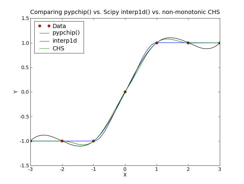
# Step function test...
#########################################################################
P.figure(2)
P.title("pchip() step function test")

# Create a step function (will demonstrate monotonicity)
x = P.arange(7.0) - 3.0
y = P.array([-1.0, -1,-1,0,1,1,1])
# Interpolate using monotonic piecewise Hermite cubic spline
xvec = P.arange(599.)/100. - 3.0
# Create the pchip slopes slopes
m = pchip_init(x,y)
# Interpolate...
yvec = pchip_eval(x, y, m, xvec)
# Call the Scipy cubic spline interpolator
from scipy.interpolate import interpolate
function = interpolate.interp1d(x, y, kind=‘cubic’)
yvec2 = function(xvec)
# Non-montonic cubic Hermite spline interpolator using

# Catmul-Rom method for computing slopes...
yvec3 =
for xx in xvec:
yvec3.append(CubicHermiteSpline(x,y,xx))
yvec3 = P.array(yvec3)
# Plot the results
P.plot(x, y, ‘ro’)
P.plot(xvec, yvec, ‘b’)
P.plot(xvec, yvec2, ‘k’)
P.plot(xvec, yvec3, ‘g’)
P.xlabel(“X”)
P.ylabel(“Y”)
P.title("Comparing pypchip() vs. Scipy interp1d() vs. non-monotonic CHS")

legends = ["Data", "pypchip()", "interp1d","CHS"]
P.legend(legends, loc=“upper left”)
P.show()
###################################################################
main()