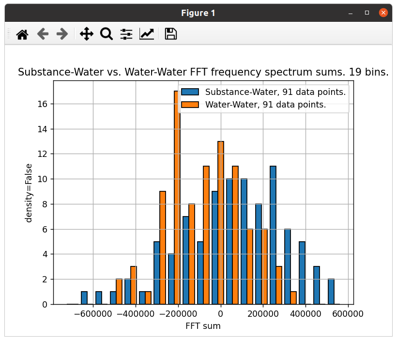
According to my logic, these 2 ways of plotting histograms of my 2 datasets should look quite similar, both they look quite different. Why?
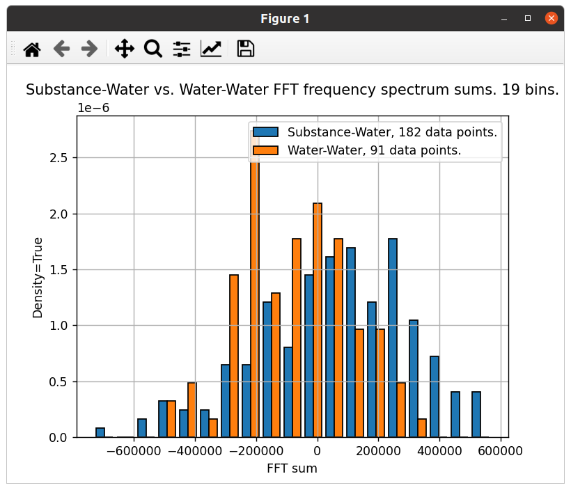
The first one is plotted with ‘density=True’, to compensate for the fact that one data set has the double number of values compared to the other:
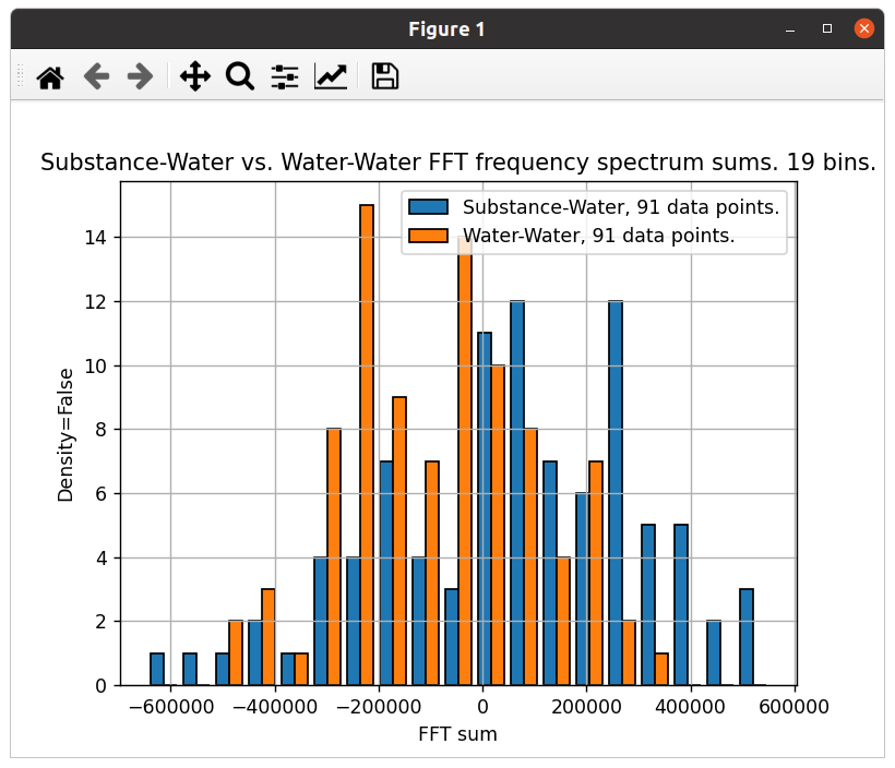
The second is plotted with ‘density=False’, but I am halving the amount of values in one data set, so the 2 data sets have the same number of values:
This is the Python code for the 2 histograms:
from matplotlib import pyplot as plot

plot.hist((sw_sums, ww_sums), edgecolor='black', bins=hist_plot_bins, density=True)
plot.title("Substance-Water vs. Water-Water FFT frequency spectrum sums. {} bins.".format(hist_plot_bins))
plot.legend(["Substance-Water, {} data points.".format(len(sw_sums)) ,"Water-Water, {} data points.".format(len(ww_sums))])
plot.xlabel('FFT sum')
plot.ylabel('density=True')
plot.grid()
plot.show()

# Since sw_sums has the double amount of elements compared to ww_sums, I average 2 at a time:
sw_sums.sort()
new_sw_sums = []
for i in range(0, len(sw_sums), 2):
    new_sw_sums.append((sw_sums[i]+sw_sums[i+1])/2)
plot.hist((new_sw_sums, ww_sums), edgecolor='black', bins=hist_plot_bins, density=False)
plot.title("Substance-Water vs. Water-Water FFT frequency spectrum sums. {} bins.".format(hist_plot_bins))
plot.legend(["Substance-Water, {} data points.".format(len(new_sw_sums)) ,"Water-Water, {} data points.".format(len(ww_sums))])
plot.xlabel('FFT sum')
plot.ylabel('density=False')
plot.grid()
plot.show()
Any explanation for the big difference between the 2 ‘density’ plots would be very appreciated. Thank you. ![]()
Here are the 2 data sets:
sw_sums= [‘-144,094.3’, ‘261,381.4’, ‘15,835.0’, ‘16,054.2’, ‘127,970.8’, ‘173,325.2’, ‘8,821.8’, ‘104,846.2’, ‘-273,515.6’, ‘-255,622.8’, ‘-182,685.4’, ‘20,458.2’, ‘-543,755.2’, ‘-329,407.9’, ‘76,067.9’, ‘-169,478.5’, ‘-169,259.3’, ‘-57,342.7’, ‘-11,988.3’, ‘-176,491.7’, ‘-80,467.3’, ‘-458,829.1’, ‘-440,936.4’, ‘-367,998.9’, ‘-164,855.3’, ‘-729,068.7’, ‘-86,308.5’, ‘319,167.3’, ‘73,620.9’, ‘73,840.1’, ‘185,756.7’, ‘231,111.1’, ‘66,607.7’, ‘162,632.1’, ‘-215,729.7’, ‘-197,837.0’, ‘-124,899.5’, ‘78,244.1’, ‘-485,969.3’, ‘-118,988.9’, ‘286,486.8’, ‘40,940.5’, ‘41,159.7’, ‘153,076.3’, ‘198,430.6’, ‘33,927.2’, ‘129,951.7’, ‘-248,410.2’, ‘-230,517.4’, ‘-157,579.9’, ‘45,563.7’, ‘-518,649.7’, ‘104,568.3’, ‘510,044.0’, ‘264,497.7’, ‘264,716.9’, ‘376,633.4’, ‘421,987.8’, ‘257,484.4’, ‘353,508.8’, ‘-24,853.0’, ‘-6,960.2’, ‘65,977.3’, ‘269,120.9’, ‘-295,092.6’, ‘-49,442.2’, ‘356,033.5’, ‘110,487.1’, ‘110,706.4’, ‘222,622.9’, ‘267,977.3’, ‘103,473.9’, ‘199,498.3’, ‘-178,863.5’, ‘-160,970.7’, ‘-88,033.3’, ‘115,110.3’, ‘-449,103.1’, ‘161,633.9’, ‘567,109.7’, ‘321,563.3’, ‘321,782.5’, ‘433,699.1’, ‘479,053.5’, ‘314,550.1’, ‘410,574.5’, ‘32,212.7’, ‘50,105.4’, ‘123,042.9’, ‘326,186.5’, ‘-238,026.9’, ‘-159,693.9’, ‘245,781.8’, ‘235.4’, ‘454.7’, ‘112,371.2’, ‘157,725.6’, ‘-6,777.8’, ‘89,246.6’, ‘-289,115.2’, ‘-271,222.4’, ‘-198,285.0’, ‘4,858.7’, ‘-559,354.8’, ‘130,789.1’, ‘536,264.8’, ‘290,718.4’, ‘290,937.7’, ‘402,854.2’, ‘448,208.6’, ‘283,705.2’, ‘379,729.6’, ‘1,367.8’, ‘19,260.6’, ‘92,198.0’, ‘295,341.6’, ‘-268,871.8’, ‘99,830.3’, ‘505,306.0’, ‘259,759.7’, ‘259,978.9’, ‘371,895.4’, ‘417,249.8’, ‘252,746.4’, ‘348,770.9’, ‘-29,591.0’, ‘-11,698.2’, ‘61,239.3’, ‘264,382.9’, ‘-299,830.6’, ‘-104,052.8’, ‘301,422.9’, ‘55,876.5’, ‘56,095.8’, ‘168,012.3’, ‘213,366.7’, ‘48,863.3’, ‘144,887.7’, ‘-233,474.1’, ‘-215,581.3’, ‘-142,643.9’, ‘60,499.7’, ‘-503,713.7’, ‘36,288.7’, ‘441,764.5’, ‘196,218.1’, ‘196,437.3’, ‘308,353.9’, ‘353,708.3’, ‘189,204.9’, ‘285,229.3’, ‘-93,132.5’, ‘-75,239.8’, ‘-2,302.3’, ‘200,841.3’, ‘-363,372.1’, ‘124,382.4’, ‘529,858.2’, ‘284,311.8’, ‘284,531.0’, ‘396,447.6’, ‘441,802.0’, ‘277,298.6’, ‘373,323.0’, ‘-5,038.8’, ‘12,853.9’, ‘85,791.4’, ‘288,935.0’, ‘-275,278.4’, ‘-51,917.2’, ‘353,558.6’, ‘108,012.2’, ‘108,231.4’, ‘220,148.0’, ‘265,502.4’, ‘100,999.0’, ‘197,023.4’, ‘-181,338.4’, ‘-163,445.7’, ‘-90,508.2’, ‘112,635.4’, ‘-451,578.0’]
ww_sums= [‘185,313.5’, ‘-57,785.9’, ‘-25,105.4’, ‘-248,662.6’, ‘-94,652.1’, ‘-305,728.3’, ‘15,599.6’, ‘-274,883.4’, ‘-243,924.6’, ‘-40,041.5’, ‘-180,383.1’, ‘-268,476.8’, ‘-92,177.2’, ‘-243,099.4’, ‘-210,419.0’, ‘-433,976.1’, ‘-279,965.6’, ‘-491,041.8’, ‘-169,713.9’, ‘-460,196.9’, ‘-429,238.1’, ‘-225,355.0’, ‘-365,696.6’, ‘-453,790.3’, ‘-277,490.7’, ‘32,680.4’, ‘-190,876.8’, ‘-36,866.2’, ‘-247,942.4’, ‘73,385.4’, ‘-217,097.5’, ‘-186,138.8’, ‘17,744.4’, ‘-122,597.2’, ‘-210,690.9’, ‘-34,391.3’, ‘-223,557.2’, ‘-69,546.7’, ‘-280,622.8’, ‘40,705.0’, ‘-249,778.0’, ‘-218,819.2’, ‘-14,936.1’, ‘-155,277.6’, ‘-243,371.3’, ‘-67,071.7’, ‘154,010.5’, ‘-57,065.6’, ‘264,262.2’, ‘-26,220.8’, ‘4,738.0’, ‘208,621.1’, ‘68,279.6’, ‘-19,814.1’, ‘156,485.4’, ‘-211,076.2’, ‘110,251.7’, ‘-180,231.3’, ‘-149,272.5’, ‘54,610.6’, ‘-85,730.9’, ‘-173,824.7’, ‘2,474.9’, ‘321,327.8’, ‘30,844.9’, ‘61,803.6’, ‘265,686.8’, ‘125,345.2’, ‘37,251.5’, ‘213,551.1’, ‘-290,483.0’, ‘-259,524.2’, ‘-55,641.1’, ‘-195,982.6’, ‘-284,076.3’, ‘-107,776.8’, ‘30,958.8’, ‘234,841.9’, ‘94,500.4’, ‘6,406.6’, ‘182,706.2’, ‘203,883.1’, ‘63,541.6’, ‘-24,552.1’, ‘151,747.4’, ‘-140,341.5’, ‘-228,435.2’, ‘-52,135.7’, ‘-88,093.7’, ‘88,205.9’, ‘176,299.6’]