Sreya
1
import numpy as np
import matplotlib.pyplot as plt
from numpy.fft import fft, ifft, fft2, fftshift
from scipy.fftpack import fftfreq, rfftfreq
total_longitude = 360
array_longitude = np.arange(0, total_longitude, 5)
hour = 72 # three days, 72 hours
array_hour = np.arange(0, hour, 1)
amplitude = 2 # amplitude
longitude = 72
frequency = 1 / 24
wavenumber = 1 / 360.0
wave = []
for i in range(0, 72):
for j in range(0, 72):
wave.append(
amplitude
* np.cos(
2 * np.pi * frequency * array_hour[i]
+ 2 * np.pi * wavenumber * array_longitude[j]
)
)
data = []
while wave != [ ]:
data.append(wave[:72])
wave = wave[72:]
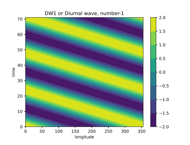
[X, Y] = np.meshgrid(array_longitude, array_hour)
Z = data[:]
fig, ax = plt.subplots(1, 1)
fp = ax.contourf(X, Y, Z)
plt.ylabel("time")
plt.xlabel("longitude")
ax.set_title("DW1 or Diurnal wave, number-1")
plt.colorbar(fp)
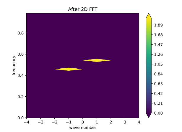
# fft
ft = np.fft.ifftshift(data)
ft1 = np.fft.fft2(ft)
ft = np.fft.fftshift(ft1)
print("+++++++++++++++++++++", ft)
feature_Y = np.arange(longitude) - longitude / 2
n=F.size
fourier_freq=np.fft.fftfreq(n, d=1.0)
print("The frequency range is, ", fourier_freq)
abs_val = np.abs(ft)
abs_val = abs_val**2
print(abs_val)
[X, Y] = np.meshgrid(feature_Y, fourier_freq)
fig, ax = plt.subplots(
1,
1,
)
Z = abs_val[:]
fp = ax.contourf(X, Y, Z, np.arange(0, (frequency + 2), 0.01), extend="both")
plt.xlim([-4, 4])
# plt.ylim([0,0.04])
fig.colorbar(fp)
plt.show()
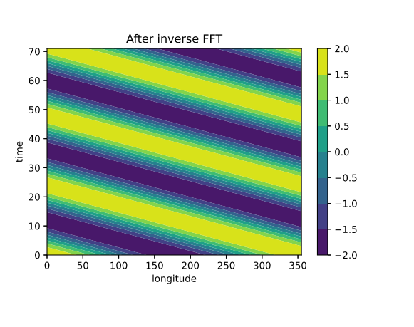
# IFFT
ift = np.fft.ifftshift(ft)
ift = np.fft.ifft2(ift)
ift = np.fft.fftshift(ift)
ift = ift.real # Take only the real part
[X, Y] = np.meshgrid(array_longitude, array_hour)
Z = ift[:]
fig, ax = plt.subplots(1, 1)
fp = ax.contourf(X, Y, Z)
plt.ylabel("time")
plt.xlabel("longitude")
ax.set_title("After inverse FFT")
plt.colorbar(fp)
plt.show()