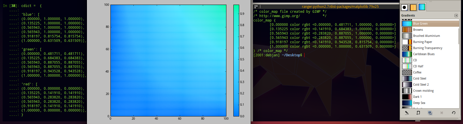
I learned some more about matplotlib colormaps from here:
http://www.scipy.org/Cookbook/Matplotlib/Show_colormaps
and tried to grasp cmap creation workflow.
Here is GMT_haxby:
_GMT_haxby_data = {
‘blue’: [
(0.0, 0.474509805441, 0.474509805441),
(0.0322580635548, 0.588235318661, 0.588235318661),
(0.0645161271095, 0.686274528503, 0.686274528503),
(0.0967741906643, 0.784313738346, 0.784313738346),
(0.129032254219, 0.831372559071, 0.831372559071),
(0.161290317774, 0.878431379795, 0.878431379795),
(0.193548381329, 0.941176474094, 0.941176474094),
(0.225806444883, 0.972549021244, 0.972549021244),
(0.258064508438, 1.0, 1.0),
(0.290322571993, 1.0, 1.0),
(0.322580635548, 1.0, 1.0),
(0.354838699102, 0.941176474094, 0.941176474094),
(0.387096762657, 0.882352948189, 0.882352948189),
(0.419354826212, 0.784313738346, 0.784313738346),
(0.451612889767, 0.68235296011, 0.68235296011),
(0.483870953321, 0.658823549747, 0.658823549747),
(0.516129016876, 0.635294139385, 0.635294139385),
(0.548387110233, 0.552941203117, 0.552941203117),
(0.580645143986, 0.474509805441, 0.474509805441),
(0.612903237343, 0.407843142748, 0.407843142748),
(0.645161271095, 0.341176480055, 0.341176480055),
(0.677419364452, 0.270588248968, 0.270588248968),
(0.709677398205, 0.29411765933, 0.29411765933),
(0.741935491562, 0.305882364511, 0.305882364511),
(0.774193525314, 0.352941185236, 0.352941185236),
(0.806451618671, 0.486274510622, 0.486274510622),
(0.838709652424, 0.61960786581, 0.61960786581),
(0.870967745781, 0.68235296011, 0.68235296011),
(0.903225779533, 0.768627464771, 0.768627464771),
(0.93548387289, 0.843137264252, 0.843137264252),
(0.967741906643, 0.921568632126, 0.921568632126),
(1.0, 1.0, 1.0)],
‘green’: [
(0.0, 0.0, 0.0),
(0.0322580635548, 0.0, 0.0),
(0.0645161271095, 0.0196078438312, 0.0196078438312),
(0.0967741906643, 0.0392156876624, 0.0392156876624),
(0.129032254219, 0.0980392172933, 0.0980392172933),
(0.161290317774, 0.156862750649, 0.156862750649),
(0.193548381329, 0.40000000596, 0.40000000596),
(0.225806444883, 0.505882382393, 0.505882382393),
(0.258064508438, 0.686274528503, 0.686274528503),
(0.290322571993, 0.745098054409, 0.745098054409),
(0.322580635548, 0.792156875134, 0.792156875134),
(0.354838699102, 0.882352948189, 0.882352948189),
(0.387096762657, 0.921568632126, 0.921568632126),
(0.419354826212, 0.921568632126, 0.921568632126),
(0.451612889767, 0.92549020052, 0.92549020052),
(0.483870953321, 0.960784316063, 0.960784316063),
(0.516129016876, 1.0, 1.0),
(0.548387110233, 0.960784316063, 0.960784316063),
(0.580645143986, 0.92549020052, 0.92549020052),
(0.612903237343, 0.843137264252, 0.843137264252),
(0.645161271095, 0.741176486015, 0.741176486015),
(0.677419364452, 0.627451002598, 0.627451002598),
(0.709677398205, 0.458823531866, 0.458823531866),
(0.741935491562, 0.313725501299, 0.313725501299),
(0.774193525314, 0.352941185236, 0.352941185236),
(0.806451618671, 0.486274510622, 0.486274510622),
(0.838709652424, 0.61960786581, 0.61960786581),
(0.870967745781, 0.701960802078, 0.701960802078),
(0.903225779533, 0.768627464771, 0.768627464771),
(0.93548387289, 0.843137264252, 0.843137264252),
(0.967741906643, 0.921568632126, 0.921568632126),
(1.0, 1.0, 1.0)],
‘red’: [
(0.0, 0.0392156876624, 0.0392156876624),
(0.0322580635548, 0.156862750649, 0.156862750649),
(0.0645161271095, 0.0784313753247, 0.0784313753247),
(0.0967741906643, 0.0, 0.0),
(0.129032254219, 0.0, 0.0),
(0.161290317774, 0.0, 0.0),
(0.193548381329, 0.101960785687, 0.101960785687),
(0.225806444883, 0.0509803928435, 0.0509803928435),
(0.258064508438, 0.0980392172933, 0.0980392172933),
(0.290322571993, 0.196078434587, 0.196078434587),
(0.322580635548, 0.266666680574, 0.266666680574),
(0.354838699102, 0.380392163992, 0.380392163992),
(0.387096762657, 0.415686279535, 0.415686279535),
(0.419354826212, 0.486274510622, 0.486274510622),
(0.451612889767, 0.541176497936, 0.541176497936),
(0.483870953321, 0.674509823322, 0.674509823322),
(0.516129016876, 0.803921580315, 0.803921580315),
(0.548387110233, 0.874509811401, 0.874509811401),
(0.580645143986, 0.941176474094, 0.941176474094),
(0.612903237343, 0.96862745285, 0.96862745285),
(0.645161271095, 1.0, 1.0),
(0.677419364452, 1.0, 1.0),
(0.709677398205, 0.956862747669, 0.956862747669),
(0.741935491562, 0.933333337307, 0.933333337307),
(0.774193525314, 1.0, 1.0),
(0.806451618671, 1.0, 1.0),
(0.838709652424, 1.0, 1.0),
(0.870967745781, 0.960784316063, 0.960784316063),
(0.903225779533, 1.0, 1.0),
(0.93548387289, 1.0, 1.0),
(0.967741906643, 1.0, 1.0),
(1.0, 1.0, 1.0)]}
Now imagine tweaking this map by hand, i.e. lower 0 value (~ 2/3 from whole cmap in example) from orange to green-blue without ruining it totally
So I want to ask this question differently: Is there some tool (Inkscape, CorelDraw, Photoshop, … anything) that would let me use GUI with some sliders so that I can try adjust matplotlib colormap?
···
On Sun, Nov 6, 2011 at 9:58 PM, klo uo <klonuo@…287…> wrote:
Like in Basemap examples:
http://matplotlib.github.com/basemap/users/examples.html (topographic
image in the middle of page) ground 0 has some yellow/orange color
making seas and oceans coasts in that same, color instead light blue
(as we’d all expect I guess)
So how to shift this particular colormap (cm.GMT_haxby) up a bit, so
that I get expected colors?