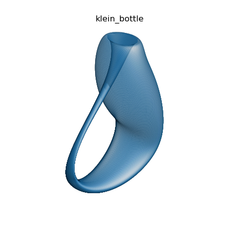
I recently included S3Dlib as a third-party package to Matplotlib. From my biased perspective ![]() , numerous examples in the documentation qualify to be in the showcase. The following is one of the simplest surface plots with the functional description given in Wikipedia.
, numerous examples in the documentation qualify to be in the showcase. The following is one of the simplest surface plots with the functional description given in Wikipedia.
import numpy as np
from matplotlib import pyplot as plt
import s3dlib.surface as s3d

# 1. Define function to examine ....................................
def klein_bottle(rtp) :
    r,v,u = rtp
    cU, sU = np.cos(u), np.sin(u)
    cV, sV = np.cos(v), np.sin(v)
    x = -(2/15)*cU* \
        (  ( 3 )*cV + \
           ( -30 + 90*np.power(cU,4) - 60*np.power(cU,6) + 5*cU*cV )*sU )
    y = -(1/15)*sU* \
        (  ( 3 - 3*np.power(cU,2) -48*np.power(cU,4) +48*np.power(cU,6) )*cV + \
           (-60 + ( 5*cU - 5*np.power(cU,3) - 80*np.power(cU,5) + 80*np.power(cU,7) )*cV  )*sU )
    z = (2/15)*( 3 + 5*cU*sU )*sV
    return x,y,z

# 2. Setup and map surface .........................................
rez=6
surface = s3d.SphericalSurface(rez)
surface.map_geom_from_op( klein_bottle, returnxyz=True )
surface.set_surface_alpha(.5)
surface.transform(s3d.eulerRot(20,-80),translate=[0,0,2])

# 3. Construct figure, add surface, show ...........................
fig = plt.figure(figsize=plt.figaspect(1))
ax = plt.axes(projection='3d')
minmax = (-1.5,1.5)
ax.set(xlim=minmax, ylim=minmax, zlim=minmax)
ax.set_axis_off()
ax.view_init(elev=20, azim=-125)
ax.set_title(surface.name)

d = [0,-1,0.5]
surface.shade(ax=ax,direction=d).hilite(ax=ax,direction=d)
ax.add_collection3d( surface )

fig.tight_layout()
plt.show()
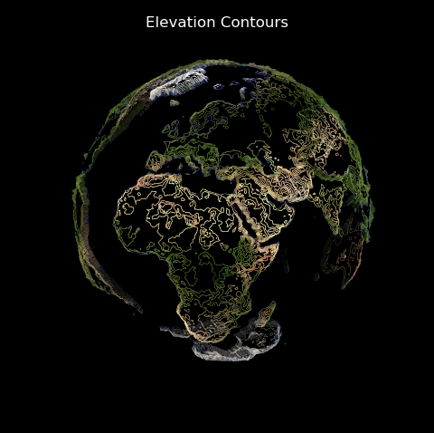
The ability to construct contours directly from surfaces is shown below, along with using images to define geometry and color.
from matplotlib import pyplot as plt
import s3dlib.surface as s3d

# 2. Setup and map surfaces .........................................
rez = 6
earth = s3d.SphericalSurface(rez,name='Elevation Contours')
earth.map_color_from_image('data/earth.png')
earth.map_geom_from_image('data/elevation.png',0.05)

elev = earth.contourLineSet(8,coor='s')
elev.set_linewidth(0.5)

# 3. Construct figure, add surface, show ............................
fig = plt.figure(figsize=plt.figaspect(1), facecolor='k' )
ax = plt.axes(projection='3d', facecolor='k')
ax.set_title(earth.name,color='w')
minmax = (-0.8,0.8)
ax.set(xlim=minmax, ylim=minmax, zlim=minmax)
ax.set_axis_off()
ax.view_init(25,-150)

ax.add_collection3d(elev.fade(ax=ax))

fig.tight_layout(pad=0)
plt.show()
The images referenced in the above script are available in the documentation. Both image sources are from the NASA visible earth catalog.
The following is a collection of several figures which were constructed ‘just of fun’. All code for these is available in the documentation examples.
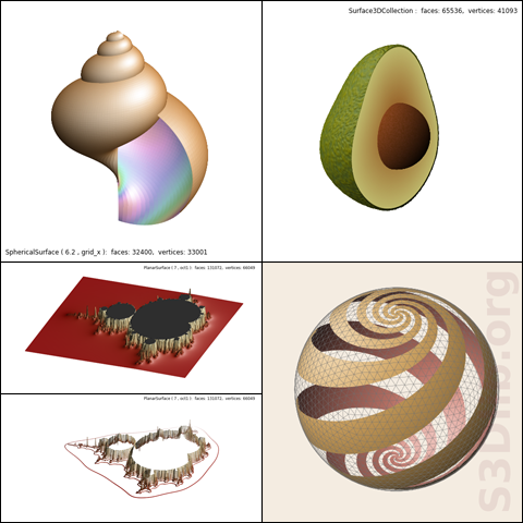
The above Mandelbrot surface S3Dlib construction used the code ‘directly’ from the Matplotlib showcase example for the functional definition.
Since S3Dlib is used to construct objects for Matplotlib rendering, animations are relatively straight forward using the matplotlib.animation module. Numerous animation examples, with code, are shown in the documentation animations examples.
I’m curious to see anyone’s ‘just for fun’ figures or ‘real-world’ application surfaces.