Hi Eric,
I think I understand the two approaches you mention, I have about the same mental distinction although with a different spin, maybe because I come from finite element/data visualisation instead of image manipulation: I see basically two type of 2D data that can be visualized as a colormapped image:
a) point data, where you provide a collection of values with associated coordinates. Algorithm is then fully responsible for computing the "best" value to associate to other coordinates (not provided by the user, but nonetheless needed to build a full image, because there was a change of resolution or just some data lacking). One can distinguish sub categories: are the points given on
- an regular rectangular grid, *
- a regular hexagonal/triangular grid,
- an irregular rectangular grid *
- another pattern? like mapped rectangular grid, ...
- at arbitrary locations, without pattern
for now in matplotlib only *-marked subcategories are supported, AFAIK
b) cell data, where you provide a collection of cell (polygons), with vertex coordinates and color-mapped data. Again we can distinguish su categories:
- cell-wise data, no interpolation needed *
- or vertex-wise data, interpolation needed
-averaging on the cell
-proximity based interpolation
-(bi)linear interpolation
-higher order interpolation
and also it can be subdivided using cell geometry criterium
- cell part of a regular rectangular grid *
- cell part of an irregular rectangular grid *
- cell part of a mapped rectangular *
- arbitray cells, but paving the plane (vertex coodinate + connectivity table)
- fully arbitrary cells, not necessarily continuously connected
Again, AFAIK for now the *-marked categories are currently suported in matplotlib.
In addition to those categories, one additional thing can be considered when any kind of interpolation/extrapolation is performed: Does the interpolation happen on the data, and then the interpolated data is mapped to color (phong mapping/interpolation/shading in matlab speach), or are is the interpolation performed on colors after the initial user-provided data have been mapped (gouraud mapping/interpolation/shading in matlab speach).
Some equivalences exists between cell based image and point based image, in particular my patch can be seen as irregular rectangular grid patches bith bilinear interpolation, or point data with bilinear interpolation. It is more of the second one, as for example in cell-data, one can expect to be able to set line styles for cell boundaries, while in point data this would have no sense.
I do not see the fact that for point data the interpolation is choosen by the algorithm as a bad thing: in fact, if one use point data, it is because there is no cell information as such, so the fact that the algorithm choose automatically the boundaries is an advantage.
For example, your NonUniformImage is a point-data image generator, which work for non-uniform rectangular grids. It associate with each pixel the data of the closest (using non-cartesian distance, but a "manhatan distance" given by abs(x-x0) + abs(y-y0)) available point data.
My patch added bilinear interpolation, using x and y bilinear interpolation between the four closest. Other type of interpolation are possible, but more complex to implement.
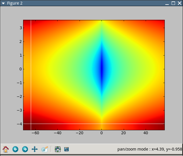
The context in which we want to use NonUniformImage is not for image processing, but for data visualisation: we have measurement data dependent on two variables (RPM and frequency), and a classic way to present such data is what is known in the field (acoustic radiation) as a "waterfall diagram". However, the samples are not necessarily taken on a regular grid. They are taken at best on an irregular grid (especially for the RPM), and at worst using a non-obvious pattern. There is no cell data here, boudaries are not really relevant, the only thing that matter is to provide an attractive and visualy-easy-to-parse image of 2D data which was sampled (or simulated) on a set of points. In this context both interpolation (nearest, usefull because if present only measured data extended in the best way so that they cover the whole figure, without any actual interpolation), and bilinear (show smoother variations, making more easy to visually detect some pattern and interresting RPM/FREQUENCY regions ) are interresting for our users...
A small example as you requested (a is withing the data, b is outside, c is completely oustide)
c
11 12 13
a b
21 22 23
31 32 33
Nearest interpolation (patched (small error), but already present):
color at a = color at 12 or 13 or 22 or 23, whichever is closest to a
color at b = color at 13 or 23, whichever is closest to b
color at c = color at 13
Bilinear interpolation (new):
S=(x23-x12)(y12-y23)
color at a = color(12) * (x23-xa)(ya-y23)/S
+ color(13) * (xa-x22)(ya-y22)/S
+ color(22) * (x13-xa)(y13-ya)/S
+ color(23) * (xa-x12)(y12-ya)/S
color at b = color(13) * (yb-y23)/(y13-y23)
+ color(23) * (y13-yb)/(y13-y23)
color at c = color at 13
As I mentioned in my first message, to complete the full array of image generation (point data, cell data, various interpolation scheme and geometric distribution of points or cell geometries, interpolation before or after the color mapping) is a tremendous work. Not even matlab has it completed, although it is far more complete than matploblib for now and can be considered a worthy goal... But I think this linear interpolation after color mapping on irregular rectangular point data is already a usefull addition 
Regards,
Greg.
Quoting Eric Firing <efiring@...229...>:
···
Grégory Lielens wrote:
Thanks a lot for reviewing my patch!
I have corrected most of the problems (I think )
I indeed introduced memory leak, I think it is fixed now, I have also
reorganized the code to avoid duplication of the cleanup code. I used an
helper function instead of the goto, because this cleanup is needed for
normal exit too, so the helper function can come in handy for that.
std::vector would have been nice, but I tried to respect the original
coding style, maybe this could be changed but I guess the original
author should have something to say about it....
Only thing I did not change is the allocation of acols/arows even when
they are not used. It is not difficult to do, but the code will be a
little more complex and I think that the extra memory used is not
significant: The memory for those mapping structure is doubled (1 float
and 1 int vector of size N, instead of a single int vector of size N),
but those mapping structures are an order of magnitude smaller than the
image buffer of size N*N of 4 char anyway...
If one agree that this is to be saved at the (slight) expense of code
conciseness/simplicity, I can add this optimisation...
Thanks for pointing the error at the left/bottom pixel lines, it is
corrected now 
And I set interpolation to NEAREST by default, so that the behavior of
NonUniformImage remains the same as before if the user do not specify
otherwise (I forgot to do it in the first patch)...
I include the new patch,
Gregory,
I am sorry to be late in joining in, but I have a basic question about
what you are trying to do. It arises from the fact that there are two
styles of image-like plots:
1) In the original Image and NonuniformImage, the colors and locations
of "pixel" (or patch or subregion or whatever) centers are specified.
2) In pcolor, quadmesh, and pcolorimage, the patch *boundaries* are
specified. pcolorimage is my modification of the original
NonuniformImage code to work with boundaries. I left the original in
place, since presumably it meets some people's needs, even though it
does not meet mine.
When the grid is uniform, it doesn't really make any difference; but
when the grid is nonuniform, then I don't think style #1 makes much
sense for pcolor-style plotting, in which there is no interpolation;
there is no unique way to specify the boundaries, so it is up to
the plotting routine, and that is bad.
For an image, it is clear how the interpolation should work: the color
values are given at the centers of the "pixels" (meaning on the original
image grid, not on the screen or other output device grid), which are
uniformly spaced, and interpolated between.
Exactly what is your patch supposed to do for the nonuniform case? Would
you describe and demonstrate it, please, for a simple case with a 2x2
array of colors and 3x3 arrays for boundary x and y?
Thanks.
Eric