Thomas Caswell <tcaswell@...149...>
writes:
The general approach follows R / seaborn / panadas and allows users to pass
in a `data` kwarg which if present, any data fields which are strings are
replaced by a call to `data[key]`. In codeax.plot(labeled_data['a'], labeled_data['b'])
and
ax.plot('a', 'b', data=labeled_data)
are equivalent.
I commented on github briefly, but here's an expanded argument. I'm
proposing that instead of using strings (or only strings) as labels, we
allow arbitrary (hashable) objects to be looked up from the data dict.
I think using strings, or at least restricting to strings only is a
mistake for two reasons. One reason has been touched upon: in
ax.scatter('a', 'b', c='b', data=data)
should c='b' be interpreted as a constant blue color or a sequence to be
looked up from data['b']?
Another is that since this functionality seems to be modeled after R's
plot functions, people will want to do more than just lookups. A simple
labeled plot in R is
plot(speed ~ dist, data=cars)
but you can also do expressions, e.g.
plot(speed^2 ~ dist, data=cars)
if you want to plot the square of speed against dist. This is pretty
neat for trying to find transformations for variables that depend on
each other non-linearly.
If we only allow strings as placeholders for plottable variables,
implementing expressions gets pretty clunky. We'd basically end up
defining a mini-language for parsing expressions from strings. But if
we allow objects for which you can implement methods like __add__,
it's much nicer. There's sample code below.
I'm proposing a small change to the patch. This still allows using
strings but also user-defined objects:
Here's a demo of implementing expressions on top of that patch:
Here's how the test case looks, and the (albeit incomplete) expression
classes and evaluator to support this are about 50 lines of pretty simple
code.
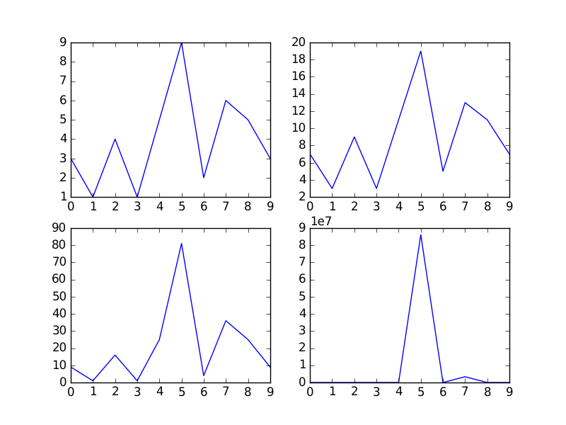
def test_expression_of_labels():
fig, axes = plt.subplots(2, 2)
x, y, z = Expr.vars('x y z')
data = {'x': np.arange(10),
'y': np.array([3, 1, 4, 1, 5, 9, 2, 6, 5, 3]),
'z': np.array([2, 7, 1, 8, 2, 8, 1, 8, 2, 8])}
ev = Evaluator(data)
axes[0, 0].plot(x, y, data=ev)
axes[0, 1].plot(x, 2 * y + 1, data=ev)
axes[1, 0].plot(x, y ** 2, data=ev)
axes[1, 1].plot(x, 2 * y ** z, data=ev)
The output: